![]()
Step 10: Perform the test
The code implemented in the previous step
[1]:
import numpy as np


class Variable:
    def __init__(self, data):
        if data is not None:
            if not isinstance(data, np.ndarray):
                raise TypeError('{} is not supported'.format(type(data)))

        self.data = data
        self.grad = None
        self.creator = None

    def set_creator(self, func):
        self.creator = func

    def backward(self):
        if self.grad is None:
            self.grad = np.ones_like(self.data)

        funcs = [self.creator]
        while funcs:
            f = funcs.pop()
            x, y = f.input, f.output
            x.grad = f.backward(y.grad)

            if x.creator is not None:
                funcs.append(x.creator)


def as_array(x):
    if np.isscalar(x):
        return np.array(x)
    return x


class Function:
    def __call__(self, input):
        x = input.data
        y = self.forward(x)
        output = Variable(as_array(y))
        output.set_creator(self)
        self.input = input
        self.output = output
        return output

    def forward(self, x):
        raise NotImplementedError()

    def backward(self, gy):
        raise NotImplementedError()


class Square(Function):
    def forward(self, x):
        y = x ** 2
        return y

    def backward(self, gy):
        x = self.input.data
        gx = 2 * x * gy
        return gx


def square(x):
    return Square()(x)


def numerical_diff(f, x, eps=1e-4):
    x0 = Variable(x.data - eps)
    x1 = Variable(x.data + eps)
    y0 = f(x0)
    y1 = f(x1)
    return (y1.data - y0.data) / (2 * eps)
Testing is an essential part of software development. Testing can help you notice mistakes (bugs) and automating testing can help you maintain the quality of your software on an ongoing basis. The same is true of the DeZero we build. This step describes how to test – specifically, how to test the Deep Learning framework.
NOTE
As software testing gets bigger, it tends to have its own ways of doing things and a lot of fiddly rules. But when it comes to testing, you don’t have to think too hard, especially at the beginning. The first thing to do is to “test it”. This step is not a “full-blown” test, but rather as simple as possible.
10.1 Unit Testing in Python
To run tests in Python, it is convenient to use unittest, which is included in the standard library. Here, let’s test the square function implemented in the previous step. The code is as follows.
[2]:
import unittest

class SquareTest(unittest.TestCase):
    def test_forward(self):
        x = Variable(np.array(2.0))
        y = square(x)
        expected = np.array(4.0)
        self.assertEqual(y.data, expected)
As above, we first import the unittest and implement the SquareTest class that extends the unittest.TestCase. The essential test is to write any method whose name starts with test and write it in it. The test we write here verifies that the output of the square function matches the expected value. Specifically, when the input is 2.0, we verify that the output is 4.0.
NOTE
In the above example, we use the method self.assertEqual to verify that the output of the square function matches the expected value. This method determines if the two given objects are equal or not. In addition to this method, unittest has various other methods, such as self.assertGreater and self.assertTrue. For other methods, see the documentation for unittest.
Now, let’s run the above test. We will assume that the above test code is in steps/step10.py. In this case, the following command can be executed from the terminal
$ python -m unittest steps/step10.py
If you are using Jupyter Notebook (or Google Colab), you can run the test with the following command.
[3]:
if __name__ == '__main__': unittest.main(argv=['first-arg-is-ignored'], exit=False)
.
----------------------------------------------------------------------
Ran 1 test in 0.004s

OK
Now, let’s check the output of the test. This output means that “we did one test and the results were OK”. This means that the test has passed. If there are any problems here, you will see output like FAIL: test_forward (step10.SquareTest) to show that the test has failed.
10.2 Testing the backward propagation of a square function
Next, let’s add a test for backward propagation of the square function. To do so, add the following code to the SquareTest class we just implemented.
[4]:
class SquareTest(unittest.TestCase):
    def test_forward(self):
        x = Variable(np.array(2.0))
        y = square(x)
        expected = np.array(4.0)
        self.assertEqual(y.data, expected)

    def test_backward(self):
        x = Variable(np.array(3.0))
        y = square(x)
        y.backward()
        expected = np.array(6.0)
        self.assertEqual(x.grad, expected)
Here, we add a method called test_backward. In it, you get the derivative by y.forward() and check whether the value of the derivative matches the expected value or not. Incidentally, the value 6.0 is set here as the expected value (expected).
Let’s test it again with the code above. As a result, we get the following output
[5]:
if __name__ == '__main__': unittest.main(argv=['first-arg-is-ignored'], exit=False)
..
----------------------------------------------------------------------
Ran 2 tests in 0.011s

OK
If you look at the results, you can see that it passed two tests. Now you can add other test cases (inputs and expected values) in the same way as before. And as the number of test cases increases, the reliability of the square function also increases. You can also repeatedly verify the state of the square function by testing it at the time you modify the code.
10.3 Automated testing with gradient check
Earlier we wrote a test for backward propagation. There, the expected value of the derivative was calculated and given by hand. In fact, there is an alternative, automatic testing method that replaces it. It’s a method called gradient check. The gradient check is performed by comparing the results obtained by numerical differentiation with the results obtained by backpropagation. If the difference is large, it is likely that there is a problem with the implementation of backpropagation.
NOTE
We implemented the numerical differentiation in “Step 4”. Numerical differentiation is easy to implement and gives you the roughly correct value of the derivative. Therefore, we can test the correctness of the back-propagation implementation by comparing it with the results of the numerical differentiation.
You only need to prepare the input values for gradient check, so you can test efficiently. So, let’s add a test by gradient check. Here, we use the numerical_diff function implemented in “Step 4”. The code for the function is also included as a review.
[6]:
def numerical_diff(f, x, eps=1e-4):
    x0 = Variable(x.data - eps)
    x1 = Variable(x.data + eps)
    y0 = f(x0)
    y1 = f(x1)
    return (y1.data - y0.data) / (2 * eps)


class SquareTest(unittest.TestCase):
    def test_forward(self):
        x = Variable(np.array(2.0))
        y = square(x)
        expected = np.array(4.0)
        self.assertEqual(y.data, expected)

    def test_backward(self):
        x = Variable(np.array(3.0))
        y = square(x)
        y.backward()
        expected = np.array(6.0)
        self.assertEqual(x.grad, expected)

    def test_gradient_check(self):
        x = Variable(np.random.rand(1))  # ランダムな入力値を生成
        y = square(x)
        y.backward()
        num_grad = numerical_diff(square, x)
        flg = np.allclose(x.grad, num_grad)
        self.assertTrue(flg)
In the test_gradient_check method for gradient check, one random input value is generated. Next, we find the derivative by back-propagation, and then the numerical differentiation by using the numerical_diff function. Then, we make sure that the values obtained by the two methods are almost identical. To do so, we use the function np.allclose of NumPy.
np.allclose(a, b) determines whether a and b of the ndarray instance are close values. How much is a “close value” can be defined by the arguments rtol and atol, as in np.allclose function(a, b, rtol=1e-05, atol=1e-08). Trueis returned if all elements ofaandbsatisfy the following conditions (|. |` denotes the absolute value).
|a - b| ≦ (atol + rtol * |b|)
The values of atol and rtol may require small adjustment depending on the calculation (function) of the gradient check. For that criterion, see, for example, literature[6]. So, let’s add the gradient check above and then run the test. This time, we get the following results.
[7]:
if __name__ == '__main__': unittest.main(argv=['first-arg-is-ignored'], exit=False)
...
----------------------------------------------------------------------
Ran 3 tests in 0.016s

OK
Thus, in the case of a deep learning framework that computes the derivatives automatically, a mechanism can be created to perform tests semi-automatically by gradient check. It allows us to systematically build test cases more broadly.
10.4 Summary of the test
When developing DeZero, the above knowledge of testing should be sufficient. You can write test code for DeZero using the steps you’ve learned here. However, in this document, we will omit the description of the test from now on. If you feel the need for test code, you can add it yourself as a reader.
In addition, it is common to keep a group of files for testing in one place. The test code are also put together in the tests directory in this book (and additional useful functions to run tests are implemented). If you’re interested, take a look at that test code. There, you’ll see a lot of code like the one I wrote in this step. In addition, the files for the test can be executed by the following command.
$ python -m unittest discover tests
You can use the sub command discover to search for test files in the directory specified after discover as above. Then, all the files found are executed together. By default, the pattern test*.py in the specified directory is recognized as a test file (this can be changed). Now you can run all the tests in the tests directory at once.
NOTE
In DeZero’s tests directory, we also run tests that take the Chainer as the correct answer. For example, to test a sigmoid function, we compute it in DeZero and Chainer for the same input, respectively, and compare whether the two outputs are almost the same value.
Also, DeZero’s GitHub repository works with a service called Travis CI, which is a service for continuous integration, and DeZero’s GitHub repository automatically runs tests when you push code or merge a pull request. Any problems with the results will be reported to you via email or other means. In addition to that, the top page of DeZero’s GitHub repository also shows a screen like Figure 10-1.
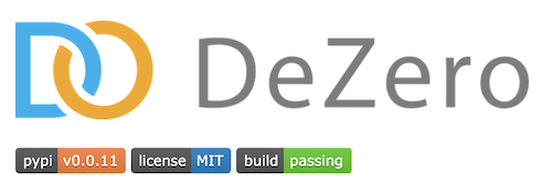
Figure 10-1 The top screen of DeZero’s GitHub repository.
As shown in Figure 10-1, you’ll see a badge that says BUILD: PASSING. This is a sign that the test has passed (if it fails, you will see a badge saying “build: failed”). By linking with CI tools like this, you can always test the source code. It helps keep the code reliable.
DeZero is a small piece of software, but we’re going to grow it into something bigger. By implementing a testing mechanism like the one described here, you can expect to maintain the reliability of your code. That’s the end of the first stage.
Little by little - and steadily - we’ve been building DeZero up to this point. The first DeZero had only “little boxes” (variables), but it has grown to the point where it can now run complex algorithms called back-propagation. For now, however, backpropagation can only be applied to simple calculations. In the next stage, we’ll extend DeZero further, so that it can be applied to more complex calculations.